![[RSS]](../theme/image/rss.png)
Space and Time not lost on the Registry
A histogram of times for which the Palomar-Leiden service has images: That's temporal service coverage right there.
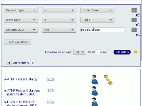
If you are an astronomer and you've ever tried looking for data in the Virtual Observatory Registry, chances are you have wondered “Why can't I enter my position here?” Or perhaps “So, I'm looking for images in [NIII] – where would I go?”
Both of these are examples for the use of Space-Time Coordinates (STC) in data discovery – yes, spectral coordinates count as STC, too, and I could make an argument for it. But this post is about something else: None of this has worked in the Registry up to now.
It's time to mend this blatant omission. To take the next steps, after a bit of discussion on some of the IVOA's mailing lists, I have posted an IVOA note proposing exactly those last Thursday. It is, perhaps with a bit of over-confidence, called A Roadmap for Space-Time Discovery in the VO Registry. And I'd much appreciate feedback, in particular if you are a VO user and have ideas on what you'd like to do with such a facility.
In this post, I'd like to give a very quick run-down on what is in it for (1) VO users, (2) service operators in general, and (3) service operators who happen to run DaCHS.
First, users. We already are pretty good on spatial coverage (for about 13000 of almost 20000 resources), so it might be worth experimenting with that. For now, the corresponding table is only available on the RegTAP mirror at http://dc.g-vo.org/tap. There, you can try queries like:
select ivoid from
rr.table_column
natural join rr.stc_spatial
where
  1=contains(gavo_simbadpoint('HDF'), coverage)
  and ucd like 'phot.flux;em.radio%'
to find – in this case – services that have radio fluxes in the area of the Hubble Deep Field. If these lines scare you or you don't know what to do with the stupid ivoids, check the previous post on this blog – it explains a bit more about RegTAP and why you might care.
Similarly cool things will, hopefully, some day be possible in spectrum and time. For instance, if you were interested in SII fluxes in the crab nebula in the early sixties, you could, some day, write:
SELECT ivoid FROM
rr.stc_temporal
NATURAL JOIN rr.stc_spectral
NATURAL JOIN rr.stc_spatial
WHERE
  1=CONTAINS(gavo_simbadpoint('M1'), coverage)
  AND 1=ivo_interval_overlaps(
    6.69e-7, 6.75e-7,
    wavelength_start, wavelength_end)
  AND 1=ivo_interval_overlaps(
    36900, 38800,
    time_start, time_end)
As you can see, the spectral coordiate will, following (admittedly broken) VO convention, be given in meters of vacuum wavelength, and time in MJD. In particular the thing with the wavelength isn't quite settled yet – personally, I'd much rather have energy there. For one, it's independent of the embedding medium, but much more excitingly, it even remains somewhat sensible when you go to non-electromagnetic messengers.
A pattern I'm trying to establish is the use of the user-defined function ivo_interval_overlaps, also defined in the Note. This is intended to allow robust query patterns in the presence of two intrinsically interval-valued things: The service's coverage and the part of the spectrum you're interested in, say. With the proposed pattern, either of these can degenerate to a single point and things still work. Things only break when both the service and you figure that “Aw, Hα is just 656.3 nm” and one of you omits a digit or adds one.
But that's academic at this point, because really few resources define their coverage in time and and spectrum. Try it yourself:
SELECT COUNT(*) FROM (
  SELECT DISTINCT ivoid FROM rr.stc_temporal) AS q
(the subquery with the DISTINCT is necessary because a single resource can have multiple rows for time and spectrum when there's multiple distinct intervals – think observation campaigns). If this gives you more than a few dozen rows when you read this, I strongly suspect it's no longer 2018.
To improve this situation, the service operators need to provide the information on the coverage in their resource records. Indeed, the registry schemas already have the notion of a coverage, and the Note, in its core, simply proposes to add three elements to the coverage element of VODataService 1.1. Two of these new elements – the coverage in time and space – are simple floating-point intervals and can be repeated in order to allow non-contiguous coverage. The third element, the spatial coverage, uses a nifty data structure called a MOC, which expands to “HEALPix Multi-Order Coverage map” and is the main reason why I claim we can now pull off STC in the Registry: MOCs let databases and other programs easily and quickly manipulate areas on the sphere. Without MOCs, that's a pain.
So, if you have registry records somewhere, please add the elements as soon as you can – if you don't know how to make a MOC: CDS' Aladin is there to help. In the end, your coverage elements should look somewhat like this:
<coverage>
  <spatial>3/336,338,450-451,651-652,659,662-663
    4/1816,1818-1819,1822-1823,1829,1840-1841</spatial>
  <temporal>37190 37250</temporal>
  <temporal>54776 54802</temporal>
  <spectral>3.3e-07 6.6e-07</spectral>
  <spectral>2.0e-05 3.5e-06</spectral>
  <waveband>Optical</waveband>
  <waveband>Infrared</waveband>
</coverage>
The waveband elements are remainders from VODataService 1.1. They are still in use (prominently, for one, in SPLAT), and it's certainly still a good idea to keep giving them for the forseeable future. You can also see how you would represent multiple observing campaigns and different spectral ranges.
Finally, if you're running DaCHS and you're using it to generate registry records (and there's almost no excuse for not doing so), you can simply write a coverage element into your RD starting with DaCHS 1.2 (or, if you run betas, 1.1.1, which is already available). You'll find lots of examples at the usual place. As a relatively interesting example, the resource descriptor of plts. It has this:
  <updater spaceTable="data" spectralTable="data" mocOrder="4"/>
  <spectral>3.3e-07 6.6e-07</spectral>
  <temporal>37190 37250</temporal>
  <temporal>38776 38802</temporal>
  <temporal>41022 41107</temporal>
  <temporal>41387 41409</temporal>
  <temporal>41936 41979</temporal>
  <temporal>43416 43454</temporal>
  <spatial>3/282,410 4/40,323,326,329,332,387,390,396,648-650,1083,1085,1087,1101-1103,1123,1125,1132-1134,1136,1138-1139,1144,1146-1147,1173-1175,1216-1217,1220,1223,1229,1231,1235-1236,1238,1240,1597,1599,1614,1634,1636,1728,1730,1737,1739-1740,1765-1766,1784,1786,2803,2807,2809,2812</spatial>
</coverage>
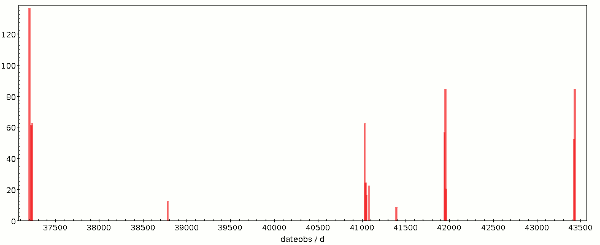
This particular service archives plate scans from the Palomar-Leiden Trojan surveys; these were looking for Trojan asteroids (of Jupiter) using the Palomar 122 cm Schmidt and were conducted in several shortish campaigns between 1960 and 1977 (incidentally, if you're looking for things near the Ecliptic, this stuff might still hold valuable insights for you). Because the fill factor for the whole time period is rather small, I manually extracted the time coverage; for that, I ran select dateobs from plts.data via TAP and made the histogram plot above. Zooming in a bit, I read off the limits in TOPCAT's coordinate display.
The other coverages, however, were put in automatically by DaCHS. That's what the updater element does: for each axis, you can say where DaCHS should look, and it will then fill in the appropriate data from what it guesses gives the relevant coordiantes – that's straightforward for standard tables like the ones behind SSAP and SIAP services (or obscore tables, for that matter), perhaps a bit more involved otherwise. To say “just do it for all axis”, give the updater a single sourceTable attribute.
Finally, in this case I'm overriding mocOrder, the order down to which DaCHS tries to resolve spatial features. I'm doing this here because in determining the coverage of image services DaCHS right now only considers the centers of the images, and that's severely underestimating the coverage here, where the data products are the beautiful large Schmidt plates. Hence, I'm lowering the resolution from the default 6 (about one degree linearly) to still give some approximation to the actual data coverage. We'll fix the underlying deficit as soon as pgsphere, the postgres extension which is actually dealing with all the MOCs, has support for turning circles and polygons into MOCs.
When you have defined an updater, just run dachs limits q.rd, and DaCHS will carefully (preserving your indentation) re-write the RD to contain what DaCHS has worked out from your table (but careful: it will overwrite what was previously there; so, make sure you only ask DaCHS to only deal with axes you're not dealing with manually).
If you feel like writing code discovering holes in the intervals, ideally already in the database: that would be great, because the tighter the intervals defined, the fewer false positives people will have in data discovery.
The take-away for DaCHS operators is:
Add STC coverage to your resources as soon as you've updated to DaCHS 1.2
If you don't have to have the tightest coverage declaration conceivable, all you have to do to have that is add:
<coverage>
  <updater sourceTable="my_table"/>
</coverage>
to your RD (where my_table is the id of your service's “main” table) and then run dachs limits q.rd
For special effects and further information, see Coverage Metadata in the DaCHS reference documentation
If you have a nice postgres function that splits a simple coverage interval up so the filling factor of a set of new intervals increases (or know a nice, database-compatible algorithm to do so) – please let me know.