Articles from Demo

  • Doing Large-Scale ADQL Queries

    You can do many interesting things with TAP and ADQL while just running queries returning a few thousand rows after a few seconds. Most examples you would find in tutorials are of that type, and when the right indexes exist on the queried tables, the scope of, let's say, casual ADQL goes far beyond toy examples.

    Actually, arranging things such that you only fetch the data you need for the analysis at hand – and that often is not much more than the couple of kilobytes that go into a plot or a regression or whatever – is a big reason why TAP and ADQL were invented in the first place.

    But there are times when the right indexes are not in place, or when you absolutely have to do something for almost everything in a large table. Database folks call that a sequential scan or seqscan for short. For larger tables (to give an order of magnitude: beyond 107 rows in my data centre, but that obviously depends), this means you have to allow for longer run times. There are even times when you may need to fetch large portions of such a large table, which means you will probably run into hard match limits when there is just no way to retrieve your full result set in one go.

    This post is about ways to deal with such situations. But let me state already that having to go these paths (in particular the partitioning we will get to towards the end of the post) may be a sign that you want to re-think what you are doing, and below I am briefly giving pointers on that, too.

    Raising the Match Limit

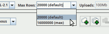
    Most TAP services will not let you retrieve arbitrarily many rows in one go. Mine, for instance, at this point will snip results off at 20'000 rows by default, mainly to protect you and your network connection against being swamped by huge results you did not expect.

    You can, and frequently will have to (even for an all-sky level 6 HEALPix map, for instance, as that will retrieve 49'152 rows), raise that match limit. In TOPCAT, that is done through a little combo box above the query input (you can enter custom values if you want):

    A screenshot with a few widgets from TOPCAT.  A combo box is opened, and the selection is on "20000 (default)".

    If you are somewhat confident that you know what you are doing, there is nothing wrong with picking the maximum limit right away. On the other hand, if you are not prepared to do something sensible with, say, two million rows, then perhaps put in a smaller limit just to be sure.

    In pyVO, which we will be using in the rest of this post, this is the maxrec argument to run_sync and its sibling methods on TAPService.

    Giving the Query More Time

    When dealing with non-trivial queries on large tables, you will often also have to give the query some extra time. On my service, for instance, you only have a few seconds of CPU time when your client uses TAP's synchronous mode (by calling TAPService.run_sync method). If your query needs more time, you will have to go async. In the simplest case, all that takes is write run_async rather than run_sync (below, we will use a somewhat more involved API; find out more about this in our pyVO course).

    In async mode, you have two hours on my box at this point; this kind of time limit is, I think, fairly typical. If even that is not enough, you can ask for more time by changing the job's execution_duration parameter (before submitting it to the database engine; you cannot change the execution duration of a running job, sorry).

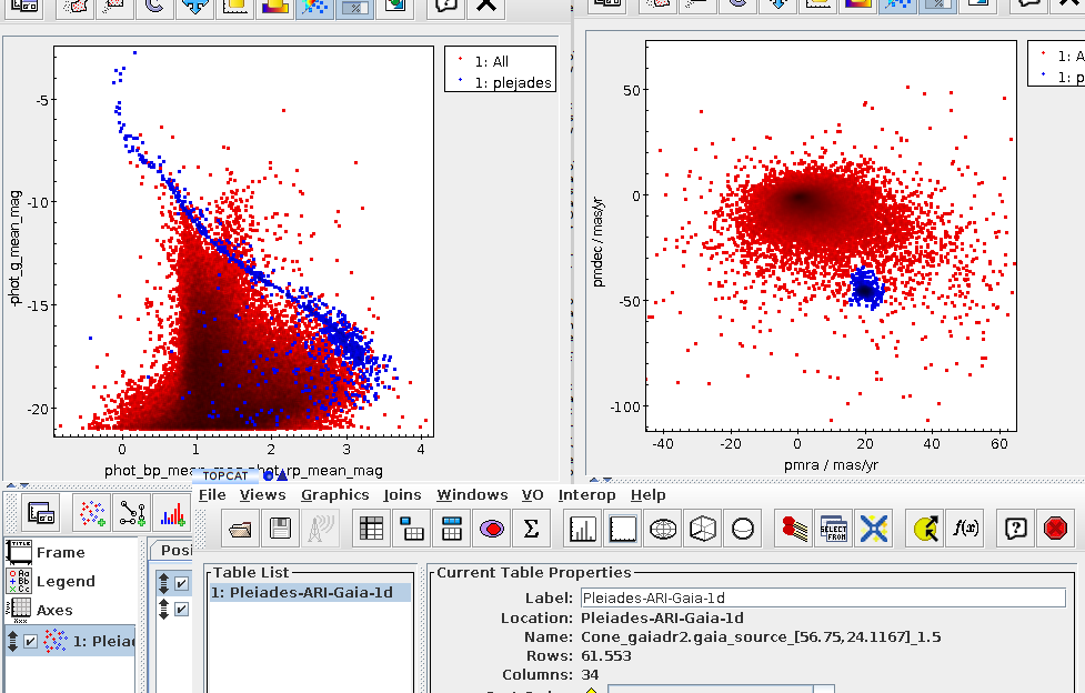
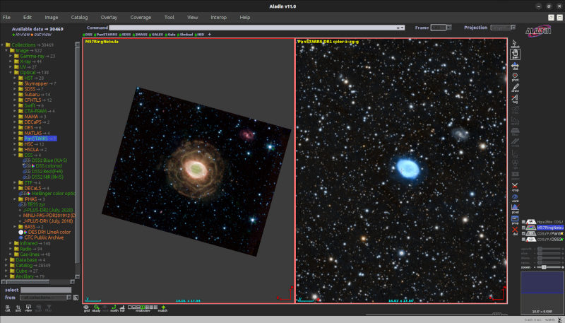
    Let us take the example of a colour-magnitude diagram for stars in Gaia DR3 with distances of about 300 pc according to Bailer-Jones et al (2021); to make things a bit more entertaining, we want to load the result in TOPCAT without first downloading it locally; instead, we will transmit the result's URI directly to TOPCAT[1], which means that your code does not have to parse and re-package the (potentially large) data.

    On the first reading, focus on the main function, though; the SAMP fun is for later:

    import time
    import pyvo
    
    QUERY = """
    SELECT
        source_id, phot_g_mean_mag, pseudocolour,
        pseudocolour_error, phot_g_mean_flux_over_error
    FROM gedr3dist.litewithdist
    WHERE
        r_med_photogeo between 290 and 310
        AND ruwe<1.4
        AND pseudocolour BETWEEN 1.0 AND 1.8
    """
    
    def send_table_url_to_topcat(conn, table_url):
        client_id = pyvo.samp.find_client_id(conn, "topcat")
        message = {
            "samp.mtype": "table.load.votable",
            "samp.params": {
                "url": table_url,
                "name": "TAP result",}
        }
        conn.notify(client_id, message)
    
    
    def main():
        svc = pyvo.dal.TAPService("http://dc.g-vo.org/tap")
        job = svc.submit_job(QUERY, maxrec=3000)
        try:
            job.execution_duration=10000  # that's 10000 seconds
            job.run()
            job.wait()
            assert job.phase=="COMPLETED"
    
            with pyvo.samp.connection(addr="127.0.0.1") as conn:
                send_table_url_to_topcat(conn, job.result_uri)
        finally:
            job.delete()
    
    if __name__=="__main__":
        main()
    

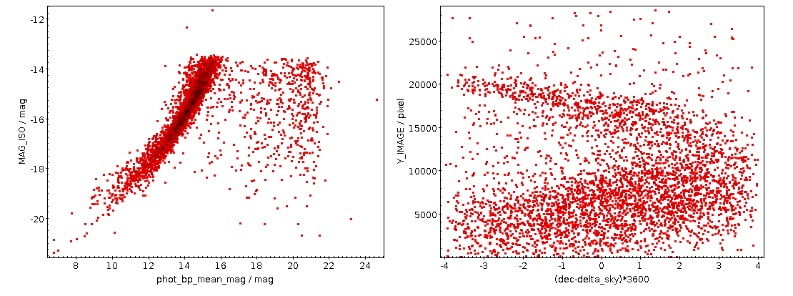
    As written, this will be fast thanks to maxrec=3000, and you wouldn't really have to bother with async just yet. The result looks nicely familiar, which means that in that distance range, the Bailer-Jones distances are pretty good:

    A rather sparsely populated colour-magnitude diagram with a pretty visible main sequence.

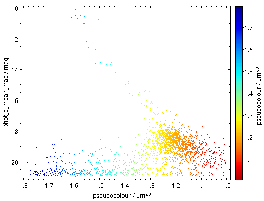
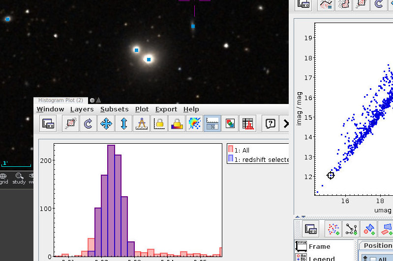
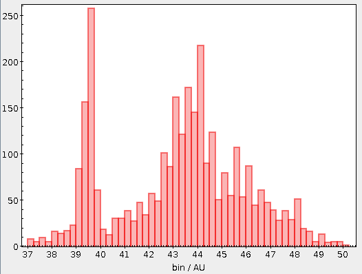
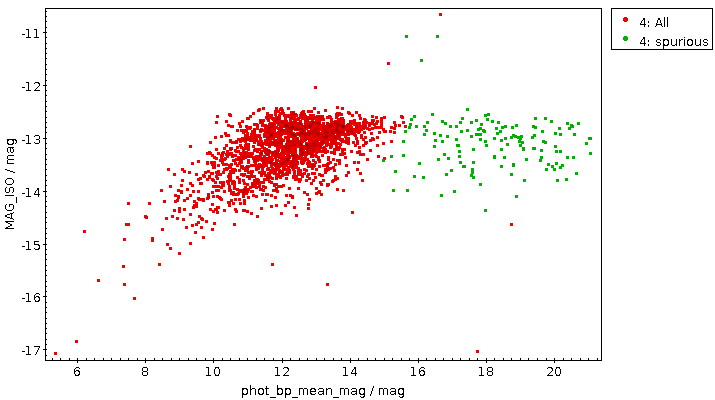
    Now raise the match limit to 30000, and you will already need async. Here is what the result looks like:

    A more densely populated colour-magnitude diagram with a pretty visible main sequence, where a giant branch starts to show up.

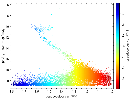
    Ha! Numbers matter: at least we are seeing a nice giant branch now! And of course the dot colours do not represent the colours of the stars with the respective pseudocolour; the directions of blue and red are ok, but most of what you are seeing here will look rather ruddy in reality.

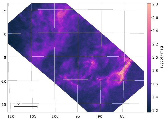
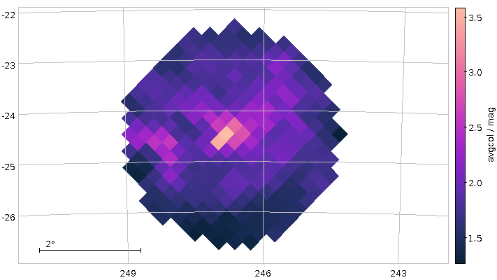
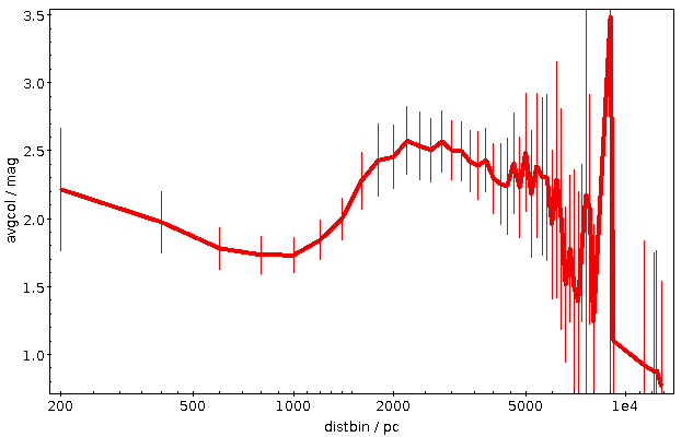
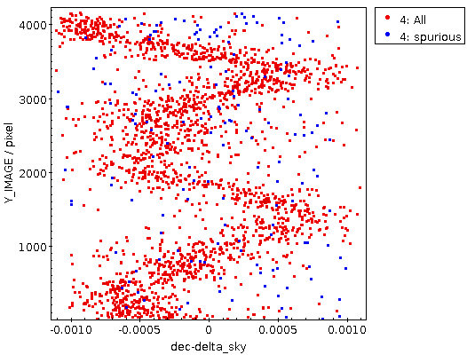
    You will not really need to change execution_duration here, nor will you need it even when setting maxrec=1000000 (or anything more, for that matter, as the full result set size is 330'545), as that ends up finishing within something like ten minutes. Incidentally, the result for the entire 300 pc shell, now as a saner density plot, looks like this:

    A full colour-magnitude diagram with densities coded in colours. A huge blob is at the red end of the main sequence, and there is a well-defined giant branch and a very visible horizontal branch.

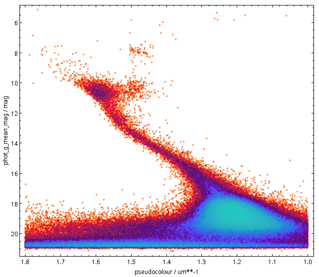
    Ha! Numbers matter even more. There is now even a (to me surprisingly clear) horizontal branch in the plot.

    Planning for Large Result Sets? Get in Contact!

    Note that if you were after a global colour-magnitude diagram as the one I have just shown, you should probably do server-side aggregation (that is: compute the densities in a few hundred or thousand bins on the server and only retrieve those then) rather than load ever larger result sets and then have the aggregation be performed by TOPCAT. More generally, it usually pays to try and optimise ADQL queries that are slow and have huge result sets before fiddling with async and, even more, with partitioning.

    Most operators will be happy to help you do that; you will find some contact information in TOPCAT's service tab, for instance. In pyVO, you could use the get_contact method of the objects you get back from the Registry API[2]:

    >>> pyvo.registry.search(ivoid="ivo://org.gavo.dc/tap")[0].get_contact()
    'GAVO Data Centre Team (+49 6221 54 1837) <gavo@ari.uni-heidelberg.de>'
    

    That said: sometimes neither optimisation nor server-side aggregation will do it: You just have to pull more rows than the service's match limit. You see, most servers will not let you pull billions of rows in one go. Mine, for instance, will cap the maxrec at 16'000'000. What you need to do if you need to pull more than that is chunking up your query such that you can process the whole sky (or whatever else huge thing makes the table large) in manageable chunks. That is called partitioning.

    Uniform-Length Partitions

    To partition a table, you first need something to partition on. In database lingo, a good thing to partition on is called a primary key, typically a reasonably short string or, even better, an integer that maps injectively to the rows (i.e., not two rows have the same key). Let's keep Gaia as an example: the primary key designed for it is the source_id.

    In the simplest case, you can “uniformly” partition between 0 and the largest source_id, which you will find by querying for the maximum:

    SELECT max(source_id) FROM gaia.dr3lite
    

    This should be fast. If it is not, then there is likely no sufficiently capable index on the column you picked, and hence your choice of the primary key probably is not a good one. This would be another reason to turn to the service's contact address as above.

    In the present case, the query is fast and yields 6917528997577384320. With that number, you can write a program like this to split up your problem into N_PART sub-problems:

    import pyvo
    
    MAX_ID, N_PART = 6917528997577384320+1, 100
    partition_limits = [(MAX_ID//N_PART)*i
      for i in range(N_PART+1)]
    
    svc = pyvo.dal.TAPService("http://dc.g-vo.org/tap")
    main_query = "SELECT count(*) FROM ({part}) AS q"
    
    for lower, upper in zip(partition_limits[:-1], partition_limits[1:]):
      result = svc.run_sync(main_query.format(part=
        "SELECT * FROM gaia.dr3lite"
        "  WHERE source_id BETWEEN {} and {} ".format(lower, upper-1)))
      print(result)
    

    Exercise: Can you see why the +1 is necessary in the MAX_ID assignment?

    This range trick will obviously not work when the primary key is a string; I would probably partition by first letter(s) in that case.

    Equal-Size Partitions

    However, this is not the end of the story. Gaia's (well thought-out) enumeration scheme reflects to a large degree sky positions. So do, by the way, the IAU conventions for object designations. Since most astronomical objects are distributed highly unevenly on the sky, creating partitions with of equal size in identifier space will yield chunks of dramatically different (a factor of 100 is not uncommon) sizes in all-sky surveys.

    In the rather common event that you have a use case in which you need a guaranteed maximum result size per partition, you will therefore have to use two passes, first figuring out the distribution of objects and then computing the desired partition from that.

    Here is an example for how one might go about this:

    from astropy import table
    import pyvo
    
    MAX_ID, ROW_TARGET = 6917528997577384320+1, 10000000
    
    ENDPOINT = "http://dc.g-vo.org/tap"
    
    # the 10000 is just the number of bins to use; make it too small, and
    # your inital bins may already overflow ROW_TARGET
    ID_DIVISOR = MAX_ID/10000
    
    DISTRIBUTION_QUERY = f"""
    select round(source_id/{ID_DIVISOR}) as bin, count(*) as ct
    from gaia.dr3lite
    group by bin
    """
    
    
    def get_bin_sizes():
      """returns a ordered sequence of (bin_center, num_objects) rows.
      """
      # since the partitioning query already is expensive, cache it,
      # and use the cache if it's there.
      try:
        with open("partitions.vot", "rb") as f:
          tbl = table.Table.read(f)
      except IOError:
        # Fetch from source; takes about 1 hour
        print("Fetching partitions from source; this will take a while"
          " (provide partitions.vot to avoid re-querying)")
        svc = pyvo.dal.TAPService(ENDPOINT)
        res = svc.run_async(DISTRIBUTION_QUERY, maxrec=1000000)
        tbl = res.table
        with open("partitions.vot", "wb") as f:
          tbl.write(output=f, format="votable")
    
      res = [(row["bin"], row["ct"]) for row in tbl]
      res.sort()
      return res
    
    
    def get_partition_limits(bin_sizes):
      """returns a list of limits of source_id ranges exhausting the whole
      catalogue.
    
      bin_sizes is what get_bin_sizes returns (and it must be sorted by
      bin center).
      """
      limits, cur_count = [0], 0
      for bin_center, bin_count in bin_sizes:
        if cur_count+bin_count>MAX_ROWS:
          limits.append(int(bin_center*ID_DIVISOR-ID_DIVISOR/2))
          cur_count = 0
        cur_count += bin_count
      limits.append(MAX_ID)
      return limits
    
    
    def get_data_for(svc, query, low, high):
      """returns a TAP result for the (simple) query in the partition
      between low and high.
    
      query needs to query the ``sample`` table.
      """
      job = svc.submit_job("WITH sample AS "
        "(SELECT * FROM gaia.dr3lite"
        "  WHERE source_id BETWEEN {} and {}) ".format(lower, upper-1)
        +query, maxrec=ROW_TARGET)
      try:
        job.run()
        job.wait()
        return job.fetch_result()
      finally:
        job.delete()
    
    
    def main():
      svc = pyvo.dal.TAPService(ENDPOINT)
      limits = get_partition_limits(get_bin_sizes())
      for ct, (low, high) in enumerate(zip(limits[:-1], limits[1:])):
        print("{}/{}".format(ct, len(limits)))
        res = get_data_for(svc, <a query over a table sample>, low, high-1)
        # do your thing here
    

    But let me stress again: If you think you need partitioning, you are probably doing it wrong. One last time: If in any sort of doubt, try the services' contact addresses.

    [1]Of course, if you are doing long-running queries, you probably will postpone the deletion of the service until you are sure you have the result wherever you want it. Me, I'd probably print the result URL (for when something goes wrong on SAMP or in TOPCAT) and a curl command line to delete the job when done. Oh, and perhaps a reminder that one ought to execute the curl command line once the data is saved.
    [2]Exposing the contact information in the service objects themselves would be a nice little project if you are looking for contributions you could make to pyVO; you would probably do a natural join between the rr.interface and the rr.res_role tables and thus go from the access URL (you generally don't have the ivoid in pyVO service objects) to the contact role.
  • Learn To Use The VO

    Thumbnails of the first 60 pages of the lecture notes, grayish goo with occasional colour spots thrown in.

    The first 60 pages of the lecture notes as they currently are. I give you a modern textbook would probably look a bit more colorful from this distance, but perhaps this will still do.

    About ten years ago, I had planned to write something I tentatively called VadeVOcum: A guide for people wanting to use the Virtual Observatory somewhat more creatively than just following and slightly adapting tutorials and use cases. If you will, I had planned to write a textbook on the VO.

    For all the usual reasons, that project never went far. Meanwhile, however, GAVO's courses on ADQL and on pyVO grew and matured. When, some time in 2021, I was asked whether I could give a semester-long course “on the VO”, I figured that would be a good opportunity to finally make the pyVO course publishable and complement the two short courses with enough framing that some coherent story would emerge, close enough to the VO textbook I had in mind in about 2012.

    Teaching Virtual Observatory Matters

    The result was a course I taught at Universität Heidelberg in the past summer semester together with Hendrik Heinl and Joachim Wambsganss. I have now published the lecture notes, which I hope are textbooky enough that they work for self-study, too. But of course I would be honoured if the material were used as a basis of similar courses in other places. To make this simpler, the sources are available on Codeberg without relevant legal restrictions (i.e., under CC0).

    The course currently comprises thirteen “lectures”. These are designed so I can present them within something like 90 minutes, leaving a bit of space for questions, contingencies, and the side tracks. You can build the slides for each of these lectures separately (see the .pres files in the source repository), which makes the PDF to work while teaching less cumbersome. In addition to that main trail, there are seven “side tracks”, which cover more fundamental or more general topics.

    In practice, I sprinkled in the side tracks when I had some time left. For instance, I showed the VOTable side track at the ends of the ADQL 2 and ADQL 3 lectures; but that really had no didactic reason, it was just about filling time. It seemed the students did not mind the topic switches to much. Still, I wonder if I should not bring at least some of the side tracks, like those on UCDs, identifiers, and vocabularies, into the main trail, as it would be unfortunate if their content fell through the cracks.

    Here is a commented table of contents:

    • Introduction: What is the VO and why should you care? (including a first demo)
    • Simple Protocols and their clients (which is about SIAP, SSAP, and SCS, as well as about TOPCAT and Aladin)
    • TAP and ADQL (that's typically three lectures going from the first SELECT to complex joins involving subqueries)
    • Interlude: HEALPix, MOC, HiPS (this would probably be where a few of the other side tracks might land, too)
    • pyVO Basics (using XService objects and a bit of SAMP, mainly along an image discovery task)
    • pyVO and TAP (which is developed around a multi-catalogue SED building case)
    • pyVO and the Registry (which, in contrast to the rest of the course, is employing Jupyter notebooks because much of the Registry API makes sense mainly in interactive use)
    • Datalink (giving a few pyVO examples for doing interesting things with the protocol)
    • Higher SAMP Magic (also introducing a bit of object oriented programming, this is mainly about tool building)
    • At the Limit: VO-Wide TAP Queries (cross-server TAP queries with query building, feature sensing and all that jazz; I admit this is fairly scary and, well, at the limit of what you'd want to show publicly)
    • Odds and Ends (other pyVO topics that don't warrant a full section)
    • Side Track: Terminology (client, server, dataset, data collection, oh my; I had expected this to grow more than it actually did)
    • Side Track: Architecture (a deeper look at why we bother with standards)
    • Side Track: Standards (a very brief overview of what standards the IVOA has produced, with a view of guiding users away from the ones they should not bother with – and perhaps towards those they may want to read after all)
    • Side Track: UCDs (including hints on how to figure out which would denote a concept one is interested in)
    • Side Track: Vocabularies (I had some doubts whether that is too much detail, but while updating the course I realised that vocabularies are now really user-visible in several places)
    • Side Track: VOTable (with the intention of giving people enough confidence to perform emergency surgery on VOTables)
    • Side Track: IVOA Identifiers (trying to explain the various ivo:// URIs users might see).

    Pitfalls: Technical, Intellectual, and Spiritual

    The course was accompanied by lab work, again 90 minutes a week. There are a few dozen exercises embedded in the course, and in the lab sessions we worked on some suitable subset of those. With the particular students I had and the lack of grading pressure, the fact that solutions for most of the exercises come with the lecture notes did not turn out to be a problem.

    The plan was that the students would explain their solutions and, more importantly, the places they got stuck in to their peers. This worked reasonably well in the ADQL part, somewhat less for the side tracks, and regrettably a lot less well in the pyVO part of the course. I cannot say I have clear lessons to be learned from that yet.

    A piece of trouble for the student-generated parts I had not expected was that the projector only interoperated with rather few of the machines the students brought. Coupling computers and projectors was occasionally difficult even in the age of universal VGA. These days, even in the unlikely event one has an adapter for the connectors on the students' computers, there is no telling what part of a computer screen will end up on the wall, which distortions and artefacts will be present and how much the whole thing will flicker.

    Oh, and better forget about trying to fix things by lowering the resolution or the refresh rate or whatever: I have not had one instance during the course in which any plausible action on the side of the computer improved the projected image. Welcome to the world of digital video signals. Next time around, I think I will bring a demonstration computer and figure out a way in which the students can quickly transfer their work there.

    Talking about unexpected technical hurdles: I am employing PDF-attached source code quite extensively in the course, and it turned out that quite a few PDF clients in use no longer do something reasonable with that. With pdf.js, I see why that would be, and it's one extra reason to want to avoid it. But even desktop readers behaved erratically, including some Windows PDF reader that had the .py extension on some sort of blacklist and refused to store the attached files on grounds that they may “damage the computer”. Ah well. I was tempted to have a side track on version control with git when writing the course. This experience is probably an encouragement to follow through with that and at least for the pyVO part to tell students to pull the files out of a checkout of the course's source code.

    Against the outline in the lecture as given, I have now promoted the former HEALPix side track to an interlude session, going between ADQL and pyVO. It logically fits there, and it was rather popular with the students. I have also moved the SAMP magic lecture to a later spot in the course; while I am still convinced it is a cool use case, and giving students a chance to get to like classes is worthwhile, too, it seems to be too much tool building to have much appeal to the average participant.

    Expectably, when doing live VO work I regularly had interesting embarrassments. For instance, in the pyvo-tap lecture, where we do something like primitive SEDs from three catalogues (SDSS, 2MASS and WISE), the optical part of the SEDs was suddenly gone in the lecture and I really wondered what I had broken. After poking at things for longer than I should have, I eventually promised to debug after class and report next time, only to notice right after the lecture that I had, to make some now-forgotten point, changed the search position – and had simply left the SDSS footprint.

    But I believe that was actually a good thing, because showing actual errors (it does not hurt if they are inadvertent) and at least brief attempts to understand them (and, possibly later, explain how one actually understood them) is a valuable part of any sort of (IT-related) education. Far too few people routinely attempt to understand what a computer is trying to tell them when it shows a message – at their peril.

    Reruns, House Calls, TV Shows

    Of course, there is a lot more one could say about the VO, even when mainly addressing users (as opposed to adopters). An obvious addition will be a lecture on the global dataset discovery API I have recently discussed here, and I plan to write it when the corresponding code will be in a pyVO release. I am also tempted to have something on stilts, perhaps in a side track. For instance, with a view to students going on to do tool development, in particular stilts' validators would deserve a few words.

    That said, and although I still did quite a bit of editing based on my experiences while teaching, I believe the material is by and large sound and up-to-date now. As I said: everyone is welcome to the material for tinkering and adoption. Hendrik and I are also open to give standalone courses on ADQL (about a day) or pyVO (two to three days) at astronomical institutes in Germany or elsewhere in not-too remote Europe as long as you house (one of) us. The complete course could be a 10-days block, but I don't think I can be booked with that[1].

    Another option would be a remote-teaching version of the course. Hendrik and I have discussed whether we have the inclination and the resources to make that happen, and if you believe something like that might fit into your curriculum, please also drop us a note.

    And of course we welcome all sorts of bug reports and pull requests on codeberg, first and foremost from people using the material to spread the VO gospel.

    [1]Well… let me hedge that I don't think I'd find a no in myself if the course took place on the Canary Islands…
  • Updates to GAVO's Tutorials

    Over the years, GAVO has produced a number of VO tutorials, i.e., texts that introduce some technique related to using the Virtual Observatory, preferably within some halfway plausible scenario. In effect, they are software documentation, and as software itself, software documentation suffers from bit rot. To work against that, the tutorials have to be revised occasionally.

    My two student assistants Sonja Gabriel and Chuanming Mao have recently done some of that revising. Let me use this opportunity to show off some of these freshly polished tutorials.

    A classic one (that has, if I may say so myself, aged rather well), is Adding catalog data to object lists using the VO. This is a thinly disguised introduction to TAP uploads, arguably the most powerful of all the VO tech to date. If you have come to this place without ever having done a TAP upload, you owe it to yourself to at least skim the tutorial and quickly follow along the few steps to do positional crossmatches with just about any astronomical catalog and with just about any level of sophistication.

    part of a screenshot: a histogram, a sky photo with overplotted points

    Another classic – it has its roots in the original Italian VO Days[1] – is TOPCAT and Aladin working together. It is using SDSS data of some galaxy cluster to try and get you to to send around data and positions between different programs using SAMP. If you are reading VO blogs, it is not unlikely this kind of thing will make you yawn. But at VO Days, it's little things like this that usually most immediately appeal to students and researchers alike.

    part of a screenshot: a color-magnitude diagram is a very narrow main sequence, and a proper motion plot

    From a tech point of view, Explore the Pleiades with TOPCAT and Aladin also mainly looks at SAMP (perhaps even somewhat less convincingly), but it's such a striking demo of what an amazing instrument Gaia is, and it's a nice introduction to TOPCAT's VO interface and subsetting facility that it's definitely worth a look, in particular as a showcase of having instant results with the VO.

    circular cloud of red crosses and blue circles in a celestial coordinate system

    An entirely different topic (well: it also employs SAMP for a moment) is covered by Data Discovery Using the Virtual Observatory Registry. This is trying to motivate looking for data collections in the VO Registry (in the form of our Browser interface to it). This tutorial has grown quite a bit during the review and now includes two sections joining data from different resources for various purposes. One section illustrates how systematics of quasar redshifts might be looked into using different sources, the other investigates the Tully-Fisher relationship in different spectral bands.

    A TOPCAT-plotted histogram with a sharp peak around 39.5 AU and a much wider one around 44.

    The tutorial on Asteroids in the Solar System was entriely overhauled. It was (and still is) mainly intended to be used in schools, and thus it originally just built on things that ran in a web browser. As is typical of things in web browsers, they have long since vanished. Hence, a rather fundamental update was necessary anyway. While we were looking for interesting things to do – the plot above, by the way, is the distribution of major halfaxes in the Kuiper belt –, we ended up even includeding a brief bit on ADQL.

    Due to its school focus, we are also offering this particular text in German as well as in English. If you are an Astronomy teacher with particularly motivated pupils , we would like to hear from you…

    An aladin window showing two aligned photos of the ring nebula in Lyra

    The last revised tutorial I would like to mention also has a somewhat special (main) target audience: Astrometric Calibration using Aladin. Admittedly, automatic, or “blind” calibration has become really great, and I think getting their images located on the sky is not much of a problem even for amateurs any more, thanks in part to services like astrometry.net. But then – sometimes there is nothing like a good, old manual, ummm, “plate” solution. Aladin and the VO make that lot less tedious than it used to be.

    Of course, I cannot have a post on tutorials without mentioning the VO Text Treasures, a web page that shows the educational material currently registered in the VO Registry. This little page also accounts for bit rot: You can sort by the time last inspected there, and thanks to Sonja's and Chuanming's efforts, our tutorials look very good in that representation at the moment.

    In case you have some material suitable for WIRR yourself: Please register it, too. Send me a mail and I will lend you a hand (or, if you are a VO pro, directly read the pertinent standard).

    [1]That's block courses on VO matters lasting a day or two. If you are in Germany, you can book us for your very own one!
  • HEALPix Maps: In General and in Gaia

    blue and reddish pixels drawing a bar on the sky.

    A map of average Gaia colours in HEALPixes 2/83 and 2/86 (Orion south-east). This post tells you how to (relatively) quickly produce such maps.

    This year's puzzler for the AG Tagung turned out to be a valuable source of interesting ADQL queries. I have already written about finding dusty spots on the sky, and in the puzzler solution, I had promised some words on creating dust maps, or, more generally, HEALPix maps of any sort.

    Making HEALPix maps with Gaia source_ids

    The basic technique is explained in Mark Taylor's classical ADASS poster from 2016. On GAVO's TAP service (access URL http://dc.g-vo.org/tap), you will also find an example for that (in TOPCAT's TAP window, check the Service-provided section unter the Examples button for it). However, once you have Gaia source_ids, there is something a lot faster and arguably not much less convenient. Let me quote the footnote on source_id from my DR3 lite table:

    For the contents of Gaia DR3, the source ID consists of a 64-bit integer, least significant bit = 1 and most significant bit = 64, comprising:

    • a HEALPix index number (sky pixel) in bits 36 - 63; by definition the smallest HEALPix index number is zero.
    • […]

    This means that the HEALpix index level 12 of a given source is contained in the most significant bits. HEALpix index of 12 and lower levels can thus be retrieved as follows:

    • [...]
    • HEALpix [at] level n = (source_id)/(235⋅412 − n).

    That is: Once you have a Gaia source_id, you an compute HEALpix indexes on levels 12 or less by a simple integer division! I give you that the more-than-35-bit numbers you have to divide by do look a bit scary – but you can always come back here for cutting and pasting:

    HEALPix level Integer-divide source id by
    12 34359738368
    11 137438953472
    10 549755813888
    9 2199023255552
    8 8796093022208
    7 35184372088832
    6 140737488355328
    5 562949953421312
    4 2251799813685248
    3 9007199254740992
    2 36028797018963968

    If you know – and that is very valuable knowledge far beyond this particular application – that you can simply jump between HEALPix indexes of different levels by multiplying with or integer-dividing by four, the general formula in the footnote actually becomes rather memorisable. Let me illustrate that with an example in Python. HEALPix number 3145 on level 6 is:

    >>> 3145//4  # ...within this HEALPix on level 5...
    786
    >>> 3145*4, (3145+1)*4  # ..and covers these on level 7...
    (12580, 12584)
    

    Simple but ingenious.

    You can immediately exploit this to make HEALPix maps like the one in the puzzler. This piece of ADQL does the job within a few seconds on the GAVO DC TAP service[1]:

    SELECT source_id/8796093022208 AS pix,
      AVG(phot_bp_mean_mag-phot_rp_mean_mag) AS avgcol
    FROM gaia.edr3lite
    WHERE distance(ra, dec, 246.7, -24.5)<2
    GROUP by pix
    

    Using the table above, you see that the horrendous 8796093022208 is the code for HEALPix level 8. When you remember (and you should) that HEALPix level 6 corresponds to a linear dimension of about 1 degree and each level is a factor of two in linear dimension, you see that the map ought to have a resolution of about 1/8th of a degree.

    HEALPix to Screen Pixel

    How do you plot this? Well, in TOPCAT, do GraphicsSky Plot, and then in the plot window LayersAdd HEALPix control (there are icons for both of these, too). You then have to manually configure the plot for the table you just retrieved: Set the Level to 8, the index to pix and the Value to avgcol – we're working on making the annotation a bit richer so that TOPCAT has a chance to figure this out by itself.

    With a bit of extra configuration, you get the following map of average colours (really: dust concentration):

    Plot: Black and reddish pixels showing a bit of structure

    This is not totally ideal, as at the border of the cone, certain Healpixes are only partially covered, which makes statistics unnecessarily harder.

    Positional Constraints using source_ids

    Due to Gaia's brilliant numbering scheme, we can do analysis by HEALpix, too, circumventing (among other things) this problem. Say you are interested in the vicinity of the M42 and would like to investigate a patch of about 8 degrees. By our rule of thumb, 8 degrees is three levels up from the one-degree level 6. To find the corresponding HEALpix index, on DaCHS servers with their gavo_simbadpoint UDF you could say:

    SELECT TOP 1 ivo_healpix_index(3, gavo_simbadpoint('M42'))
    FROM tap_schema.tables
    

    Hu, you ask, what's tap_schema.tables to do with this? Well, nothing, really. It's just that ADQL's syntax requires selecting from a table, even if what we select is completely independent of any table, as for instance the index of M42's 3-HEALpix. The hack above picks in a table guaranteed to exist on all TAP services, and the TOP 1 makes sure we only compute the value once. In case you ever feel the need to abuse a TAP service as a calculator: Keep this trick in mind.

    The result, 334, you could also have found more graphically, as follows:

    1. Start Aladin
    2. Check OverlayHEALPix grid
    3. Enter M42 in Command
    4. Zoom out until you see HEALPix indexes of level 3 in the grid.

    An advantage you have with this method: You see that M42 happens to lie on a border of HEALPixes; perhaps you should include all of 334, 335, 356, and 357 if you were really interested in the Orion Nebula's vicinity.

    We, on the other hand, are just interested in instructive examples, and hence let's just repeat our colour mapping with all Gaia objects from HEALPix 3/334. How do you select these? Well, by source_id's construction, you know their source_ids will be between 334⋅9007199254740992 and (334 + 1)⋅9007199254740992 − 1:

    SELECT source_id/8796093022208 AS pix,
      AVG(phot_bp_mean_mag-phot_rp_mean_mag) AS avgcol
    FROM gaia.edr3lite
    WHERE source_id BETWEEN 334*9007199254740992 AND 335*9007199254740992-1
    GROUP by pix
    

    This is computationally cheap (though Postgres, not being a column store still has to do quite a bit of I/O; note how much faster this query is when you run it again and all the tuples are already in memory). Even going to HEALPix level 2 would in general still be within our sync time limit. The opening figure was produced with the constraint:

    source_id BETWEEN 83*36028797018963968 AND 84*36028797018963968-1
    OR source_id BETWEEN 86*36028797018963968 AND 87*36028797018963968-1
    

    – and with a sync query.

    Aggregating over a Non-HEALPix

    One last point: The constraints we have just been using are, in effect, positional constraints. You can also use them as quick and in some sense rather unbiased sampling tools.

    For instance, if you would like so see how the reddening in one of the “dense“ spots in the opening picture behaves with distance, you could first pick a point – α = 98, δ = 4, say –, then convert that to a level 7 healpix as above (that's/88974) and then write:

    SELECT ROUND(r_med_photogeo/200)*200 AS distbin, COUNT(*) as n,
        AVG(phot_bp_mean_mag-phot_rp_mean_mag) AS avgcol
    FROM gaia.dr3lite
    JOIN gedr3dist.main USING (source_id)
    WHERE source_id BETWEEN 88974*35184372088832 and 88975*35184372088832-1
    GROUP BY distbin
    

    This is creating 200 pc bins in distance based on the estimates in the gedr3dist.main table (note that this adds subtle correlations, because these estimates already contain Gaia colour information). Since quite a few of these bins will be very sparsely populated, I'm also fetching the number of objects contributing. And then I plot the whole thing, using the conventional (n) ⁄ n as a rough estimate for the relative error:

    Plot: A line that first slowly declines, then rises quite a bit, then flattens out and becomes crazy as errors start to dominate.

    This plot immediatly shows that colour systematics are not exclusively due to dust, as in that case things would only get redder all the time. The blueward trend up to 700 pc is reasonably well explained by the brighter, bluer upper main sequence becoming more dominant in the population sampled as red dwarfs become too faint for Gaia.

    The strong reddening setting in after that is rather certainly due to the Orion complex, though I would perhaps not have expected it to reach out to 2 kpc (the conventional distance to M42 is about 0.5 kpc); without having properly thought about it, I'll chalk it off as “the Orion arm“. And after that, it's again what I'd call Malmquist-blueing until the whole things dissolves into noise.

    In conclusion: Did you know you can group by both healpix and distbin at the same time? I am sure there are interesting structures to be found in what you will get from such a query…

    [1]You may be tempted to write source_id/(POWER(2, 35)*POWER(4, 3) here for clarity. Resist that temptation. POWER returns floating point numbers. If you have one float in a division, not even a ROUND will get you back into the integer division realm, and the whole trick implodes. No, you will need the integer literals for now.
  • Computing Residuals of an Astrometric Calibration

    Two plots, left a fairly good correlation, right a cloudy wave

    The kind of plot you can make following the recipe given here: Left, a comparison of the photometry, right, a positional residuals, not taking into account the SIP plate solution, when comparing the HDAP plate B3261a against Gaia DR3. Note that the cut-off a 4 arcsec is because of the match radius when obtaining the calibrator stars.

    I recently had to assess the quality of the astrometric calibration of a photographic plate. What I am going to show you in this post will of course work just as well for CCD frames, and if these have a sufficiently large field of view, this may be an issue for them as well. However, the sort of data that needs this assessment most typically are scans of plates, as these tend to have a “wobble”, systematic offsets in the scan direction resulting from imperfections in the mechanics.

    Prerequisites: An astronomical frame with a calibration in ICRS (or some frame not very far from it), called my-image.fits in the following, SExtractor (in Debian and derivatives: apt install source-extractor – long live Debian Astro; since it's called source-extractor in Debian, that's what I'll use here, too), and of course TOPCAT.

    Step 1: Extract Sources. Source extraction is of course a high science, and if you know better than me, by all means do it the way you think is appropriate. Meanwhile, the following might very well work for you sufficiently well.

    Create a working directory and enter it. Then, to create a file telling source-extractor what columns you would like to see, write the following to a file default.param:

    ALPHA_SKY
    DELTA_SKY
    X_IMAGE
    Y_IMAGE
    MAG_ISO
    FLUX_AUTO
    ELONGATION
    

    Next, give a few parameters to source-extractor; depending on the sort of image you have, you may want to play around with DETECT_MINAREA (how many pixels need to show a signal to register as a source) and DETECT_THRESH (how many sigmas a pixel has to be above the background to register as a candidate for belonging to a source). Meanwhile, write the following into a file default.control:

    CATALOG_TYPE     FITS_1.0
    CATALOG_NAME     img.axy
    PARAMETERS_NAME  default.param
    FILTER           N
    DETECT_MINAREA   30
    DETECT_THRESH    4
    SEEING_FWHM      1.2
    

    – but if the following call gives you a few hundred sources, that ought to work for the present purpose.

    Then run:

    source-extractor -c default.control my-image.fits
    

    This will give you a catalogue of extracted objects in the file img.axy.

    Step 2: Fix source-extractor's output. Load that img.axy into TOPCAT. Regrettably, source-extractor does not add any useful metadata to the columns of its output table. To add the absolute bare minimum, in TOPCAT go to ViewsColumn Info. In that window, check UCD in the Display menu, and then put pos.eq.ra and pos.eq.dec into the UCD fields of the ALPHA_SKY and DELTA_SKY columns, respectively; double click to change fields in TOPCAT.

    To see if you have done the annotation right, in TOPCAT's main window, click GraphicsSky Plot. If the objects show up, you have just provided enough annotation to let TOPCAT figure out the position for each row.

    Step 3: Get calibrators. We will now try to add counterparts for Gaia DR3 to the extracted sources. To do that, click VOTable Access Protocol, and in the window popping up double click the entry for the GAVO DC TAP.

    In the Find box, type dr3lite to look for this site's version of the Gaia DR3 source catalogue. Click on gaia.dr3lite to select that table, and then select the Columns pane. This should show some of the Gaia DR3 columns.

    Now ExamplesUpload Join will generate a query that will cross-match your extracted sources with the Gaia sources. You should edit it a bit, only selecting the columns you will actually need, removing the TOP 1000 (at least on large images with more than 1000 sources), and reducing the match radius a bit when the calibration is not actually completely off and your epoch is sufficiently close to J2000.

    Hint: you can control-click in the Columns pane and then use the Cols button to insert all the column names in one go[1]. For me, the resulting query would be:

    SELECT
       source_id, ra, dec, phot_bp_mean_mag,
       tc.*
       FROM gaia.dr3lite AS db
       JOIN TAP_UPLOAD.t1 AS tc
       ON 1=CONTAINS(POINT('ICRS', db.ra, db.dec),
                     CIRCLE('ICRS', tc.ALPHA_SKY, tc.DELTA_SKY, 4./3600.))
    

    This should result in about as many matches as your extraction had – a few more is ok, because you will have some spurious matches, a few less is ok, too, as there are always some outliers and artefacts, but you should clearly not pull a magnitude more or less objects here than you put in; fiddle with the match radius as necessary.

    See if there is a rough correlation between the Gaia calibrators and your extracted sources by plotting phot_bp_mean_mag against MAG_ISO. Absent more information, MAG_ISO, source-extractor's guess for the magnitude of the extracted object, will be just some crazy number, but it should have some discernable correlation with the actual magnitude. Do not expect too much here, in particular with old plates, for which good photometry is a science of their own.

    In my example, this looked like this:

    Plot: a rough correlation in red with a green tail

    The green points certainly are spurious matches; this observation did not reach beyond 14th magnitude or so, and there are many weak stars on the sky, so a few of them will show up in just about any cross match. See the opening picture for an example with a better correlation.

    Step 4: Do the correlation plot. Do GraphicsPlane Plot and then plot ra-alpha_sky or dec-delta_sky against X_IMAGE or Y_IMAGE. You could get something like this:

    Plot: A single wavy thing

    This rather certainly reflects some optical distortion; source-extractor regrettably does not take into account SIP corrections yet, so it is likely that a large part of this would be taken care of by the polynomials of the plate solution (the github issue I am linking to tells you how to be sure).

    But it can also look like this:

    Plot: Multiple wobbles

    This certainly is not the result of a lens or anything optical at all. It's the scanner's gears that you are looking at here. With an amplitude of perhaps three arcseconds this is rather excessive here; but something like this you will rather likely see even on good scanners – though it may essentially be invisible, as of the Heidelberg scanner we used for HDAP:

    Plot: A vertical cloud with no discernible structure.
    [1]I'm using the BP magnitude in the query below as most historical plates tend to be “blue sensitive“ (in some sense). Hence, BP magnitudes should be a bit closer to what source-extractor has extracted.

Page 1 / 4 »