• GAVO at the AG-Tagung in Köln

    People standing an sitting around a booth-like table.  There's a big GAVO logo and a big screen on the left-hand side, a guy in a red hoodie is clearly giving a demo.

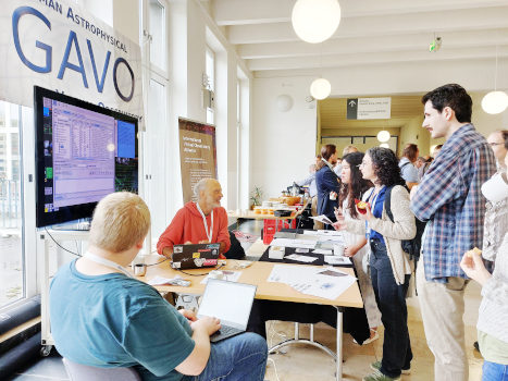
    As every year, GAVO participates in the fall meeting of the Astronomische Gesellschaft (AG), the association of astronomers working in Germany. This year, the meeting is hosted by the Universität zu Köln (a.k.a. University of Cologne), and I want to start with thanking them and the AG staff for placing our traditional booth smack next to a coffee break table. I anticipate with glee our opportunities to run our pitches on how much everyone is missing out if they're not doing VO while people are queueing up for coffee. Excellent.

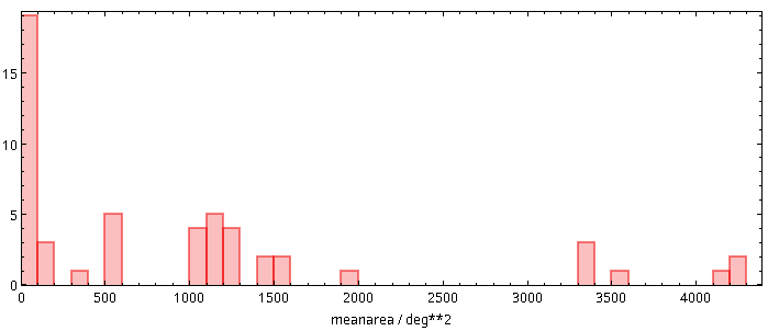
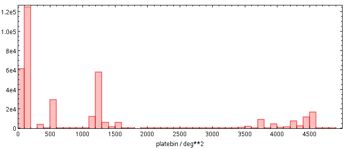
    As every year, we are co-conveners for a splinter meeting on e-science the virtual observatory, where I will be giving a talk on global dataset discovery (you heard it here first; lecture notes for the talk) late on Thursday afternoon.

    And as every year, there is a puzzler, a little problem rather easily solvable using VO tools; I was delighted to see people apparently already waiting for it when I handed out the problem sheet during the welcome reception tonight. You are very welcome to try your hand on it, but you only get to enter our raffle if you are on site. This year, the prize is a towel (of course) featuring a great image from ESA's Mars Express mission, where Phobos floats in front of Mars' limb:

    A 2:1 landscape black-and-white image with a blackish irregular spheroid floating in front of a deep horizon.

    I will update this post with the hints we are going to give out during the coffee breaks tomorrow and on Wednesday. And I will post our solution here late on Thursday.

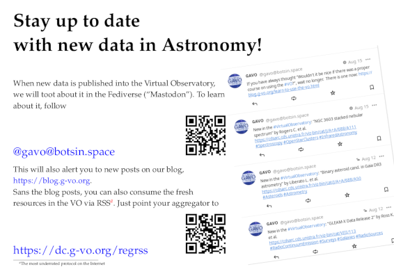
    At our booth, you will also find various propaganda material, mostly covering matters I have mentioned here before; for posteriority and remoteriority, let me link to PDFs of the flyers/posters I have made for this meeting (with re-usabilty in mind). To advertise the new VO lectures, I am asking Have you ever wished there was a proper introduction to using the Virtual Observatory? with lots of cool DOIs and perhaps less-cool QR codes. Another flyer trying to gain street cred with QR codes is the Follow us flyer advertising our Fediverse presence. We also still show a pitch for publishing with us and hand out the inevitable who we are flyer (which, I'll readily admit, has never been an easy sell).

    A fediverse screenshot and URIs for following us.

    Bonferroni for Open Data?

    A lot more feedback than on the QR code-heavy posters I got on a real classic that I have shown at many AG meetings since the 2013 Tübingen meeting: Lame excuses for not publishing data.

    A tricky piece of feedback on that was an excuse that may actually be a (marginally) valid criticism of open data in general. You see, in particular in astroparticle physics (where folks are usually particularly uptight with their data), people run elaborate statistics on their results, inspired by the sort of statistics they do in high energy physics (“this is a 5-sigma detection of the Higgs particle”). When you do this kind of thing, you do run into a problem when people run new “tests” against your data because of the way test theory works. If you are actually talking about significance levels, you would have to apply Bonferroni corrections (or worse) when you do new tests on old data.

    This is actually at least not untrue. If you do not account for the slight abuse of data and tests of this sort, the usual interpretation of the significance level – more or less the probablity that you will reject a true null hypothesis and thus claim a spurious result – breaks down, and you can no longer claim things like “aw, at my significance level of 0.05, I'll do spurious claims only one out of twenty times tops”.

    Is this something people opening their data would need to worry about when they do their original analysis? It seems obvious to me that that's not the case and it would actually be impossible to do, in particular given that there is no way to predict what people will do in the future. But then there are many non-obvious results in statistics going against at least my gut feelings.

    Mind you, this definitely does not apply to most astronomical research and data re-use I have seen. But the point did make me wonder whether we may actually need some more elaborate test theory for re-used open data. If you know about anything like that: please do let me know.

    Followup (2024-09-10)

    The first hint is out. It's “Try TOPCAT's TAP client to solve this puzzler; you may want to took for 2MASS XSC there.“ Oh, and we noticed that the problem was stated rather awkwardly in the original puzzler, which is why we have issued an erratum. The online version is fixed, it now says “where we define obscure as covered by a circle of four J-magnitude half-light radii around an extended object”.

    Followup (2024-09-10)

    After our first splinter – with lively discussions on the concept and viability of the “science-ready data” we have always had in mind as the primary sort of thing you would discover in the VO –, I have revealed the second hint: “TOPCAT's Examples button is always a good idea, in particular if you are not too proficient in ADQL. What you would need here is known as a Cone Selection.”

    Oh, in case you are curious where the discussion on the science-ready data gyrated to: Well, while the plan for supplying data usable without having to have reduction pipelines in place is a good one. However, there undoubtedly are cases in which transparent provenance and the ability to do one's own re-reductions enable important science. With datalink [I am linking to a 2015 poster on that written by me; don't read that spec just for fun], we have an important ingredient for that. But I give you that in particular the preservation of the software that makes up reduction pipelines is a hard problem. It may even be an impossible problem if “preservation” is supposed to encompass malleability and fixability.

    Followup (2024-09-11)

    I've given the last two hints today: “To find the column with the J half-light radius, it pays to sort the columns in the Columns tab in TOPCAT by name or, for experts using VizieR's version of the XSC, by UCD.” and “ADQL has aggregate functions, which let you avoid downloading a lot of data when all you need are summary properties. This may not matter with what little data you would transfer here, but still: use server-side SUM.”

    Followup (2024-09-12)

    I have published the (to me, physically surprising) puzzler solution to https://www.g-vo.org/puzzlerweb/puzzler2024-solution.pdf. In case it matters to you: The towel went to Marburg again. Congratulations to the winner!

    Followup (2024-09-13)

    On the way home I notice this might be a suitable place to say how I did the QR codes I was joking about above. Basis: The embedding documents are written in LaTeX, and I'm using make to build them. To include a QR code, I am writing something like:

    \includegraphics[height=5cm]{vo-qr.png}}
    

    in the LaTeX source, and I am declaring a dependency on that file in the makefile:

    fluggi.pdf: fluggi.tex vo-qr.png <and possibly more images>
    

    Of course, this will error out because there is no file vo-qr.png at that point. The plan is to programatically generate it from a file containing the URL (or whatever you want to put into the QR code), named, in this case, vo.url (that is, whatever is in front of -qr.png in the image name). In this case, this has:

    https://doi.org/10.21938/avVAxDlGOiu0Byv7NOZCsQ
    

    The automatic image generation then is effected by a pattern rule in the makefile:

    %-qr.png: %.url
            python qrmake.py $<
    

    And then all it takes is a short script qrmake.py, which based on python3-qrcode:

    import sys
    import qrcode
    
    with open(sys.argv[1], "rb") as f:
            content = f.read().strip()
    output_code = qrcode.QRCode(border=0)
    output_code.add_data(content)
    
    dest_name = sys.argv[1].replace(".url", "")+"-qr.png"
    output_code.make_image().save(dest_name)
    
  • Learn To Use The VO

    Thumbnails of the first 60 pages of the lecture notes, grayish goo with occasional colour spots thrown in.

    The first 60 pages of the lecture notes as they currently are. I give you a modern textbook would probably look a bit more colorful from this distance, but perhaps this will still do.

    About ten years ago, I had planned to write something I tentatively called VadeVOcum: A guide for people wanting to use the Virtual Observatory somewhat more creatively than just following and slightly adapting tutorials and use cases. If you will, I had planned to write a textbook on the VO.

    For all the usual reasons, that project never went far. Meanwhile, however, GAVO's courses on ADQL and on pyVO grew and matured. When, some time in 2021, I was asked whether I could give a semester-long course “on the VO”, I figured that would be a good opportunity to finally make the pyVO course publishable and complement the two short courses with enough framing that some coherent story would emerge, close enough to the VO textbook I had in mind in about 2012.

    Teaching Virtual Observatory Matters

    The result was a course I taught at Universität Heidelberg in the past summer semester together with Hendrik Heinl and Joachim Wambsganss. I have now published the lecture notes, which I hope are textbooky enough that they work for self-study, too. But of course I would be honoured if the material were used as a basis of similar courses in other places. To make this simpler, the sources are available on Codeberg without relevant legal restrictions (i.e., under CC0).

    The course currently comprises thirteen “lectures”. These are designed so I can present them within something like 90 minutes, leaving a bit of space for questions, contingencies, and the side tracks. You can build the slides for each of these lectures separately (see the .pres files in the source repository), which makes the PDF to work while teaching less cumbersome. In addition to that main trail, there are seven “side tracks”, which cover more fundamental or more general topics.

    In practice, I sprinkled in the side tracks when I had some time left. For instance, I showed the VOTable side track at the ends of the ADQL 2 and ADQL 3 lectures; but that really had no didactic reason, it was just about filling time. It seemed the students did not mind the topic switches to much. Still, I wonder if I should not bring at least some of the side tracks, like those on UCDs, identifiers, and vocabularies, into the main trail, as it would be unfortunate if their content fell through the cracks.

    Here is a commented table of contents:

    • Introduction: What is the VO and why should you care? (including a first demo)
    • Simple Protocols and their clients (which is about SIAP, SSAP, and SCS, as well as about TOPCAT and Aladin)
    • TAP and ADQL (that's typically three lectures going from the first SELECT to complex joins involving subqueries)
    • Interlude: HEALPix, MOC, HiPS (this would probably be where a few of the other side tracks might land, too)
    • pyVO Basics (using XService objects and a bit of SAMP, mainly along an image discovery task)
    • pyVO and TAP (which is developed around a multi-catalogue SED building case)
    • pyVO and the Registry (which, in contrast to the rest of the course, is employing Jupyter notebooks because much of the Registry API makes sense mainly in interactive use)
    • Datalink (giving a few pyVO examples for doing interesting things with the protocol)
    • Higher SAMP Magic (also introducing a bit of object oriented programming, this is mainly about tool building)
    • At the Limit: VO-Wide TAP Queries (cross-server TAP queries with query building, feature sensing and all that jazz; I admit this is fairly scary and, well, at the limit of what you'd want to show publicly)
    • Odds and Ends (other pyVO topics that don't warrant a full section)
    • Side Track: Terminology (client, server, dataset, data collection, oh my; I had expected this to grow more than it actually did)
    • Side Track: Architecture (a deeper look at why we bother with standards)
    • Side Track: Standards (a very brief overview of what standards the IVOA has produced, with a view of guiding users away from the ones they should not bother with – and perhaps towards those they may want to read after all)
    • Side Track: UCDs (including hints on how to figure out which would denote a concept one is interested in)
    • Side Track: Vocabularies (I had some doubts whether that is too much detail, but while updating the course I realised that vocabularies are now really user-visible in several places)
    • Side Track: VOTable (with the intention of giving people enough confidence to perform emergency surgery on VOTables)
    • Side Track: IVOA Identifiers (trying to explain the various ivo:// URIs users might see).

    Pitfalls: Technical, Intellectual, and Spiritual

    The course was accompanied by lab work, again 90 minutes a week. There are a few dozen exercises embedded in the course, and in the lab sessions we worked on some suitable subset of those. With the particular students I had and the lack of grading pressure, the fact that solutions for most of the exercises come with the lecture notes did not turn out to be a problem.

    The plan was that the students would explain their solutions and, more importantly, the places they got stuck in to their peers. This worked reasonably well in the ADQL part, somewhat less for the side tracks, and regrettably a lot less well in the pyVO part of the course. I cannot say I have clear lessons to be learned from that yet.

    A piece of trouble for the student-generated parts I had not expected was that the projector only interoperated with rather few of the machines the students brought. Coupling computers and projectors was occasionally difficult even in the age of universal VGA. These days, even in the unlikely event one has an adapter for the connectors on the students' computers, there is no telling what part of a computer screen will end up on the wall, which distortions and artefacts will be present and how much the whole thing will flicker.

    Oh, and better forget about trying to fix things by lowering the resolution or the refresh rate or whatever: I have not had one instance during the course in which any plausible action on the side of the computer improved the projected image. Welcome to the world of digital video signals. Next time around, I think I will bring a demonstration computer and figure out a way in which the students can quickly transfer their work there.

    Talking about unexpected technical hurdles: I am employing PDF-attached source code quite extensively in the course, and it turned out that quite a few PDF clients in use no longer do something reasonable with that. With pdf.js, I see why that would be, and it's one extra reason to want to avoid it. But even desktop readers behaved erratically, including some Windows PDF reader that had the .py extension on some sort of blacklist and refused to store the attached files on grounds that they may “damage the computer”. Ah well. I was tempted to have a side track on version control with git when writing the course. This experience is probably an encouragement to follow through with that and at least for the pyVO part to tell students to pull the files out of a checkout of the course's source code.

    Against the outline in the lecture as given, I have now promoted the former HEALPix side track to an interlude session, going between ADQL and pyVO. It logically fits there, and it was rather popular with the students. I have also moved the SAMP magic lecture to a later spot in the course; while I am still convinced it is a cool use case, and giving students a chance to get to like classes is worthwhile, too, it seems to be too much tool building to have much appeal to the average participant.

    Expectably, when doing live VO work I regularly had interesting embarrassments. For instance, in the pyvo-tap lecture, where we do something like primitive SEDs from three catalogues (SDSS, 2MASS and WISE), the optical part of the SEDs was suddenly gone in the lecture and I really wondered what I had broken. After poking at things for longer than I should have, I eventually promised to debug after class and report next time, only to notice right after the lecture that I had, to make some now-forgotten point, changed the search position – and had simply left the SDSS footprint.

    But I believe that was actually a good thing, because showing actual errors (it does not hurt if they are inadvertent) and at least brief attempts to understand them (and, possibly later, explain how one actually understood them) is a valuable part of any sort of (IT-related) education. Far too few people routinely attempt to understand what a computer is trying to tell them when it shows a message – at their peril.

    Reruns, House Calls, TV Shows

    Of course, there is a lot more one could say about the VO, even when mainly addressing users (as opposed to adopters). An obvious addition will be a lecture on the global dataset discovery API I have recently discussed here, and I plan to write it when the corresponding code will be in a pyVO release. I am also tempted to have something on stilts, perhaps in a side track. For instance, with a view to students going on to do tool development, in particular stilts' validators would deserve a few words.

    That said, and although I still did quite a bit of editing based on my experiences while teaching, I believe the material is by and large sound and up-to-date now. As I said: everyone is welcome to the material for tinkering and adoption. Hendrik and I are also open to give standalone courses on ADQL (about a day) or pyVO (two to three days) at astronomical institutes in Germany or elsewhere in not-too remote Europe as long as you house (one of) us. The complete course could be a 10-days block, but I don't think I can be booked with that[1].

    Another option would be a remote-teaching version of the course. Hendrik and I have discussed whether we have the inclination and the resources to make that happen, and if you believe something like that might fit into your curriculum, please also drop us a note.

    And of course we welcome all sorts of bug reports and pull requests on codeberg, first and foremost from people using the material to spread the VO gospel.

    [1]Well… let me hedge that I don't think I'd find a no in myself if the course took place on the Canary Islands…
  • What's new in DaCHS 2.10

    A part of the IVOA product-type vocabulary, and the DaCHS logo with a 2.10 behind it.

    About twice a year, I release a new version of our VO server package DaCHS; in keeping with tradition, this post summarises some of the more notable changes of the most recent release, DaCHS 2.10.

    productTypeServed

    The next version of VODataService will probably have a new element for service descriptions: productTypeServed. This allows operators to declare what sort of files will come out of a service: images, time series, spectra, or some of the more exotic stuff found in the IVOA product-type vocabulary (you can of course give multiple of these). More on where this is supposed to go is found my Interop talk on this. DaCHS 2.10 now lets you declare what to put there using a productTypeServed meta item.

    For SIA and SSAP services, there is usually no need to give it, as RegTAP services will infer the right value from the service type. But if you serve, say, time series from SSAP, you can override the inference by saying something like:

    <meta name="productTypeServed">timeseries</meta>
    

    Where this really is important is in obscore, because you can serve any sort of product through a single obscore table. While you could manually declare what you serve by overriding obscore-extraevents in your userconfig RD, this may be brittle and will almost certainly get out of date. Instead, you can run dachs limits //obscore (and you should do that occasionally anyway if you have an obscore table). DaCHS will then feed the meta from what is in your table.

    A related change is that where a piece of metadata is supposed to be drawn from a vocabulary, dachs val will now complain if you use some other identifier. As of DaCHS 2.10 the only metadata item controlled in this way is productTypeServed, though.

    Registering Obscore Tables

    Speaking about Obscore: I have long been unhappy about the way we register Obscore tables. Until now, they rode piggyback in the registry record of the TAP services they were queriable through. That was marignally acceptable as long as we did not have much VOResource metadata specific to the Obscore table. In the meantime, we have coverage in space, time, and spectrum, and there are several meaningful relationships that may be different for the obscore table than for the TAP service. And since 2019, we have the Discovering Data Collections Note that gives a sensible way to write dedicated registry records for obscore tables.

    With the global dataset discovery (discussed here in February) that should come with pyVO 1.6 (and of course the productTypeServed thing just discussed), there even is a fairly pressing operational reason for having these dedicated obscore records. There is a draft of a longer treatment on the background on github (pre-built here) that I will probably upload into the IVOA document repository once the global discovery code has been merged. Incidentally, reviews of that draft before publication are most welcome.

    But what this really means: If you have an obscore table, please run dachs pub //obscore after upgrading (and don't forget to run dachs limits //obscore after you do notable changes to your obscore table).

    Ranking

    Arguably the biggest single usability problem of the VO is <drumroll> sorting! Indeed, it is safe to assume that when someone types “Gaia DR3“ into any sort of search mask, they would like to find some way to query Gaia's gaia_source table (and then perhaps all kinds of other things, but that should reasonably be sorted below even mirrors of gaia_source. Regrettably, something like that is really hard to work out across the Registry outside of these very special cases.

    Within a data centre, however, you can sensibly give an order to things. For DaCHS, that in particular concerns the order of tables in TAP clients and the order of the various entries on the root page. For instance, a recent TOPCAT will show the table browser on the GAVO data centre like this:

    Screenshot of a hierachical display, top-level entries are, in that order, ivoa, tap_schema, bgds, califadr3; ivoa is opened and shows obscore and obs_radio, califadr3 is opened and shows cubes first, then fluxpos tables and finally flux tables.

    The idea is that obscore and TAP metadata are way up, followed by some data collections with (presumably) high scientific value for which we are the primary site; within the califadr3 schema, the tables are again sorted by relevance, as most people will be interested in the cubes first, the somewhat funky fluxpos tables second, and in the entirely nerdy flux tables last.

    You can arrange this by assigning schema-rank metadata at the top level of an RD, and table-rank metadata to individual tables. In both cases, missing ranks default to 10'000, and the lower a rank, the higher up a schema or table will be shown. For instance, dfbsspec/q (if you wonder what that might be: see Byurakan to L2) has:

    <resource schema="dfbsspec">
      <meta name="schema-rank">100</meta>
        ...
        <table id="spectra" onDisk="True" adql="True">
          <meta name="table-rank">1</meta>
    

    This will put dfbsspec fairly high up on the root page, and the spectra table above all others in the RD (which have the implicit table rank of 10'000).

    Note that to make DaCHS notice your rank, you need to dachs pub the modified RDs so the ranks end up in DaCHS' dc.resources table; since the Registry does not much care for these ranks, this is a classic use case for the -k option that preserves the registry timestamp of the resource and will thus prevent a re-publication of the registry record (which wouldn't be a disaster either, but let's be good citizens). Ideally, you assign schema ranks to all the resources you care about in one go and then just say:

    dachs pub -k ALL
    

    The Obscore Radio Extension

    While the details are still being discussed, there will be a radio extension to Obscore, and DaCHS 2.10 contains a prototype implementation for the current state of the specification (or my reading of it). Technically, it comprises a few columns useful for, in particular, interferometry data. If you have such data, take a look at https://github.com/ivoa-std/ObsCoreExtensionForRadioData.git and then consider trying what DaCHS has to offer so far; now is the time to intervene if something in the standard is not quite the way it should be (from your perspective).

    The documentation for what to do in DaCHS is a bit scarce yet – in particular, there is no tutorial chapter on obs-radio, nor will there be until the extension has converged a bit more –, but if you know DaCHS' obscore support, you will be immediately at home with the //obs-radio#publish mixin, and you can see it in (very limited) action in the emi/q RD.

    The FITS Media Type

    I have for a long time recommended to use a media type of image/fits for FITS “images” and application/fits for FITS (binary) tables. This was in gross violation of standards: I had freely invented image/fits, and you are not supposed to invent media types without then registering them with the IANA.

    To be honest, the invention was not mine (only). There are applications out there flinging around image/fits types, too, but never mind: It's still bad practice, and DaCHS 2.10 tries to rectify it by first using application/fits even where defaults have been image/fits before, and actually retroactively changing image/fits to application/fits in the database where it can figure out that a column contains a media type.

    It is accepting image/fits as an alias for application/fits in SIAP's FORMAT parameter, and so I hope nothing will break. You may have to adapt a few regression tests, though.

    On the Way To pathlib.Path

    For quite a while, Python has had the pathlib module, which is actually quite nice; for instance, it lets you write dir / name rather than os.path.join(dir, name). I would like to slowly migrate towards Path-s in DaCHS, and thus when you ask DaCHS' configuration system for paths (something like base.getConfig("inputsDir")), you will now get such Path-s.

    Most operator code, however, is still isolated from that change; in particular, the sourceToken you see in grammars mostly remains a string, and I do not expect that to change for the forseeable future. This is mainly because the usual string operations many people to do remove extensions and the like (self.sourceToken[:-5]) will fail rather messily with Path-s:

    >>> n = pathlib.Path("/a/b/c.fits")
    >>> n[:-5]
    Traceback (most recent call last):
      File "<stdin>", line 1, in <module>
    TypeError: 'PosixPath' object is not subscriptable
    

    So, if you don't call getConfig in any of your DaCHS-facing code, you are probably safe. If you do and get exceptions like this, you know where they come from. The solution, stringification, is rather straightforward:

    >>> str(n)[:-5]
    '/a/b/c'
    

    Partly as a consequence of this, there were slight changes in the way processors work. I hope I have not damaged anyone's code, but if you do custom previews and you overrode classify, you will have to fix your code, as that now takes an accref together with the path to be created.

    Odds And Ends

    As usual, there are many minor improvements and additions in DaCHS. Let me mention security.txt support. This complies to RFC 9116 and is supposed to give folks discovering a vulnerability a halfway reliable way to figure out who to complain to. If you try http://<your-hostname>/.well-known/security.txt, you will see exactly what is in https://dc.g-vo.org/.well-known/security.txt. If this is in conflict with some bone-headed security rules your institution may have, you can replace security.txt in DaCHS' central template directory (most likely /usr/lib/python3/dist-packages/gavo/resources/templates/); but in that case please complain, and we will make this less of a hassle to change or turn off.

    You can no longer use dachs serve start and dachs serve stop on systemd boxes (i.e., almost all modern Linux boxes as configured by default). That is because systemd really likes to manage daemons itself, and it gets cross when DaCHS tries to do it itself.

    Also, it used to be possible to fetch datasets using /getproduct?key=some/accref. This was a remainder of some ancient design mistake, and DaCHS has not produced such links for twelve years. I have now removed DaCHS' ability to fetch accrefs from key parameters (the accrefs have been in the path forever, as in /getproduct/some/accref). I consider it unlikely that someone is bitten by this change, but I personally had to fix two ancient regression tests.

    If you use embedded grammars and so far did not like the error messages because they always said “unknown location“, there is help: just set self.location to some string you want to see when something is wrong with your source. For illustration, when your source token is the name of a text file you process line by line, you would write:

    <iterator><code>
      with open(self.sourceToken) as f:
        for line_no, line in enumerate(f):
          self.location = f"{self.sourceToken}, {line_no}"
          # not do whatever you need to do on line
    </code></iterator>
    

    When regression-testing datalink endpoints, self.datalinkBySemantics may come in handy. This returns a mapping from concept identifiers to lists of matching rows (which often is just one). I have caught myself re-implementing what it does in the tests itself once too often.

    Finally, and also datalink-related, when using the //soda#fromStandardPubDID descriptor generator, you sometimes want to add just an extra attribute or two, and defining a new descriptor generator class for that seems too much work. Well, you can now define a function addExtras(descriptor) in the setup element and mangle the descriptor in whatever way you like.

    For instance, I recently wanted to enrich the descriptor with a few items from the underlying database table, and hence I wrote:

    <descriptorGenerator procDef="//soda#fromStandardPubDID">
      <bind name="accrefPrefix">"dasch/q/"</bind>
      <bind name="contentQualifier">"image"</bind>
      <setup>
        <code>
          def addExtras(descriptor):
            descriptor.suppressAutoLinks = True
            with base.getTableConn() as conn:
              descriptor.extMeta = next(conn.queryToDicts(
                "SELECT * FROM dasch.plates"
                " WHERE obs_publisher_did = %(did)s",
                {"did": descriptor.pubDID}))
        </code>
      </setup>
    </descriptorGenerator>
    

    Upgrade As Convenient

    That's it for the notable changes in DaCHS 2.10. As usual, if you have the GAVO repository enabled, the upgrade will happen as part of your normal Debian apt upgrade. Still, if you have not done so recently, have a quick look at upgrading in the tutorial. If, on the other hand, you use the Debian-distributed DaCHS package and you do not need any of the new features, you can let things sit and enjoy the new features after your next dist-upgrade.

    Oh, by the way: If you are still on buster (or some other distribution that still has astropy 4): A few (from my perspective minor) things will be broken; astropy is evolving too fast, but in general, I am trying to hack around the changes to make DaCHS work at least with the astropys in oldstable, stable, and unstable. However, in cases when a failure seems to be more of an annoyance to, I am resigning. If any of the broken things do bother you, do let me know, but also consider installing a backport of astropy 5 or higher – or, better, to dist-upgrade to bookworm. Sorry about that.

  • Watch Sphinx Doctests

    No astronomy at all here; please move on if tooling for improving tooling bores you.

    While giving a lecture on pyVO, I am churning out quite a few pull requests against pyVO at the moment. I am also normally also fairly religious about running unit tests before doing a commit. But then PyVO unit tests became really, really slow a while ago when pytesting of the examples in the documentation was turned on, and so I started relying on the github continuous integration, which feels fairly wasteful – and also makes all kinds of minor idiocies public that I would have caught locally with a test suite that finishes within a minute or so.

    Regrettably, tooling for inspecting how doctests with sphinx and pytest run is not really great: All the code from one documentation file translates into a single test, and when that runs for five minutes, it's anyone's guess where the time is spent. After a bit of poking and asking around, it seemed to me that there indeed is no “doctest profiler” (if you will), at least not for pytest-executable doctests embedded in sphinx-processable ReStructuredText.

    Well, I thought, let's write a quick one. Originally, I had wanted to use the docutils parser for robustness, but once I tried to pull in the sphinx extensions and got lost in their modules I decided a simple, RE-based parser has to be enough.

    And here it is, my my quick-and-dirty doctest profiler: watch-doctests.py. Just put it into your path, make it executable, and you can do something like this:

    pyvo/docs/dal > watch-doctests.py index.rst | head -30
    ---0.00---------------
    
    import pyvo as vo
    ---0.94---------------
    
    service = vo.dal.SIAService("http://dc.zah.uni-heidelberg.de/lswscans/res/positions/siap/siap.xml")
    ---0.94---------------
    
    print(service.description)
    Scans of plates kept at Landessternwarte Heidelberg-Königstuhl. They
    were obtained at location, at the German-Spanish Astronomical Center
    (Calar Alto Observatory), Spain, and at La Silla, Chile. The plates
    cover a time span between 1880 and 1999.
    
    Specifically, HDAP is essentially complete for the plates taken with
    the Bruce telescope, the Walz reflector, and Wolf's Doppelastrograph
    at both the original location in Heidelberg and its later home on
    Königstuhl.
    ---1.02---------------
    
    import pyvo as vo
    ---1.02---------------
    
    from astropy.coordinates import SkyCoord
    ---1.02---------------
    
    from astropy.units import Quantity
    

    – so, you pass in the ReStructuredText with the embedded sphinx/pytest doctests, and then the thing extracts every line to be executed in the doctests (it ignores the outputs, so it will not actually check any assertions), prints the runtime so far in a separator and then runs the code through Python as usual: note that no automatic repr() of any non-None results – that the REPL does – happens. This is for profiling, not for test development.

    The quick hack helped me speed up the dal and registry doctests by sizeable factors, for instance because I am now avoiding downloads of large datasets, and I am using faster queries where I can.

    So, that's nice. But unless someone asks, I will distribute the code here only and in this ad-hoc fashion (probably with a link in the pyVO hackers' docs). I still believe there must be something a lot less hacky that does about the same thing somewhere out there…

  • A Data Publisher's Diary: Wide Images in DASCH

    An Aladin screenshot with many green squares overplotted on a DSS image sized 20×15 degrees.

    This is the new resonse when you query the DASCH SIAP service for Aladin's default view on the horsehead nebula. As you can see, at least the returned images no longer are distributed over half of the sky (note the size of the view).

    The first reaction I got when the new DASCH in the VO service hit Aladin was: “your SIAP service is broken, it just dumps all images it has at me rather than honouring my positional constraint.”

    I have to admit I was intially confused as well when an in-view search from Aladin came back with images with centres on almost half the sky as shown in my DASCH-in-Aladin illustration. But no, the computer did the right thing. The matching images in fact did have pixels in the field of view. They were just really wide field exposures, made to “patrol” large parts of the sky or to count meteors.

    DASCH's own web interface keeps these plates out of the casual users' views, too. I am following this example now by having two tables, dasch.narrow_plates (the “narrow” here follows DASCH's nomenclature; of course, most plates in there would still count as wide-field in most other contexts) and dasch.wide_plates. And because the wide plates are probably not very helpful to modern mainstream astronomers, only the narrow plates are searched by the SIAP2 service, and only they are included with obscore.

    In addition to giving you a little glimpse into the decisions one has to make when running a data centre, I wrote this post because making a provisional (in the end, I will follow DASCH's classification, of course) split betwenn “wide” and “narrow” plates involved a bit of simple ADQL that may still be not totally obvious and hence may merit a few words.

    My first realisation was that the problem is less one of pixel scale (it might also be) but of the large coverage. How do we figure out the coverage of the various instruments? Well, to be robust against errors in the astrometric calibration (these happen), let us average; and average over the area of the polygon we have in s_region, for which there is a convenient ADQL function. That is:

    SELECT instrument_name, avg(area(s_region)) as meanarea
    FROM dasch.plates
    GROUP BY instrument_name
    

    It is the power of ADQL aggregate function that for this characterisation of the data, you only need to download a few kilobytes, the equivalent of the following histogram and table:

    A histogram with a peak of about 20 at zero, with groups of bars going all the way beyond 4000.  The abscissa is marked “meanarea/deg**2”.
    Instrument Name mean size [sqdeg]
    Eastman Aero-Ektar K-24 Lens on a K-1...  
    Cerro Tololo 4 meter  
    Logbook Only. Pages without plates.  
    Roe 6-inch  
    Palomar Sky Survey (POSS)  
    1.5 inch Ross (short focus) 4284.199799877725
    Patrol cameras 4220.802442888225
    1.5-inch Ross-Xpress 4198.678060743206
    2.8-inch Kodak Aero-Ektar 3520.3257323233624
    KE Camera with Installed Rough Focus 3387.5206396388453
    Eastman Aero-Ektar K-24 Lens on a K-1... 3370.5283986677637
    Eastman Aero-Ektar K-24 Lens on a K-1... 3365.539790633015
    3 inch Perkin-Zeiss Lens 1966.1600884072298
    3 inch Ross-Tessar Lens 1529.7113188540836
    2.6-inch Zeiss-Tessar 1516.7996790591587
    Air Force Camera 1420.6928219265849
    K-19 Air Force Camera 1414.074101143854
    1.5 in Cooke "Long Focus" 1220.3028263587332
    1 in Cook Lens #832 Series renamed fr... 1215.1434235932702
    1-inch 1209.8102811770807
    1.5-inch Cooke Lenses 1209.7721123964636
    2.5 inch Cooke Lens 1160.1641223648048
    2.5-inch Ross Portrait Lens 1137.0908812243645
    Damons South Yellow 1106.5016573891376
    Damons South Red 1103.327982978934
    Damons North Red 1101.8455616455205
    Damons North Blue 1093.8380971825375
    Damons North Yellow 1092.9407550755682
    New Cooke Lens 1087.918570304363
    Damons South Blue 1081.7800084709982
    2.5 inch Voigtlander (Little Bache or... 548.7147592220762
    NULL 534.9269386355818
    3-inch Ross Fecker 529.9219051692568
    3-inch Ross 506.6278856912204
    3-inch Elmer Ross 503.7932693652602
    4-inch Ross Lundin 310.7279860552893
    4-inch Cooke (1-327) 132.690621660727
    4-inch Cooke Lens 129.39637516917298
    8-inch Bache Doublet 113.96821604869973
    10-inch Metcalf Triplet 99.24964308212328
    4-inch Voightlander Lens 98.07368690379751
    8-inch Draper Doublet 94.57937153909593
    8-inch Ross Lundin 94.5685388440282
    8-inch Brashear Lens 37.40061588712761
    16-inch Metcalf Doublet (Refigured af... 33.61565584978583
    24-33 in Jewett Schmidt 32.95324914757339
    Asiago Observatory 92/67 cm Schmidt 32.71623733985344
    12-inch Metcalf Doublet 31.35112644688316
    24-inch Bruce Doublet 22.10390937657793
    7.5-inch Cooke/Clark Refractor at Mar... 14.625992810622787
    Positives 12.600189007151709
    YSO Double Astrograph 10.770798601877804
    32-36 inch BakerSchmidt 10 1/2 inch r... 10.675406541122827
    13-inch Boyden Refractor 6.409447066606171
    11-inch Draper Refractor 5.134521254785461
    24-inch Clark Reflector 3.191361603405415
    Lowel 40 inch reflector 1.213284257086087
    200 inch Hale Telescope 0.18792105301170514

    For the instruments with an empty mean size, no astrometric calibrations have been created yet. To get a feeling for what these numbers mean, recall that the celestial sphere has an area of 4 π rad², that is, 4⋅180²/π or 42'000 square degrees. So, some instruments here indeed covered 20% of the night sky in one go.

    I was undecided between cutting at 150 (there is a fairly pronounced gap there) or at 50 (the gap there is even more pronounced) square degrees and provisionally went for 150 (note that this might still change in the coming days), mainly because of the distribution of the plates.

    You see, the histogram above is about instruments. To assess the consequences of choosing one cut or the other, I would like to know how many images a given cut will remove from our SIAP and ObsTAP services. Well, aggregate functions to the rescue again:

    SELECT ROUND(AREA(s_region)/100)*100 AS platebin, count(*) AS ct
    FROM dasch.plates
    GROUP BY platebin
    

    To plot such a pre-computed histogram in TOPCAT, tell the histogram plot window to use ct as the weight, and you will see something like this:

    A wide histogram with a high peak at about 50, rising to 1.2e5. Another noticeable concentration is around 1250, and there is signifiant weight also approaching 450 from the left.

    It was this histogram that made me pick 150 deg² as the cutoff point for what should be discoverable in all-VO queries: I simply wanted to retain the plates in the second bar from left.

« Page 2 / 21 »